Exploring Moving Average Trading Strategies With Mathematica
A common technical indicator you’ll find on sites such as Google Finance and Morning Star is the moving average. This represents the average value of the stock around a set period relative to a particular day. The following chart shows the world stock market (MSCI World) with the 120 day moving average (blue) and the 30 day moving average (red):
Clean[a_] := #/First[#] &@(#[[2]] & /@ a); (* extract closing data *)
dateRange = {"2009-01-01", "2012-12-30"};
ClippedMovingAverage[n_, m_, series_] :=
  Drop[Drop[MovingAverage[series, n], Floor[(n - m)/2]],
    Floor[(m - n)/2]];

vt = Clean[FinancialData["VT", dateRange]];
ma30 = ClippedMovingAverage[30, 120, vt];
ma120 = ClippedMovingAverage[120, 120, vt];
ma1 = ClippedMovingAverage[1, 120, vt];

graph = ListLinePlot[{ma1, ma30, ma120},
  PlotStyle -> {{Black, Thin}, {Red, Thick}, {Blue, Thick}},
  ImageSize -> {500}]
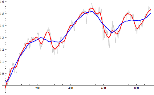
We can see that the moving averages cross when the index experiences sharp rises and falls.
The Strategy
The idea is to use this as an indicator that the index has momentum in a particular direction and signals that you should either get into a position or exit a position depending on the direction. Lets see how much money we could have made implementing this strategy. First we’ll need to create a signal to tell us when to buy and when to sell. We’ll define this signal as 1 on days we should buy or hold,and 0 on days we should sell or keep our cash:
signal = If[# >= 0, 1, 0] & /@ (ma30 - ma120);
graph = ListLinePlot[{ma1, ma30, ma120, signal},
  PlotStyle -> {{Black, Thin}, {Red, Thick}, {Blue, Thick}, {Black,
      Thick}}, ImageSize -> {500}]
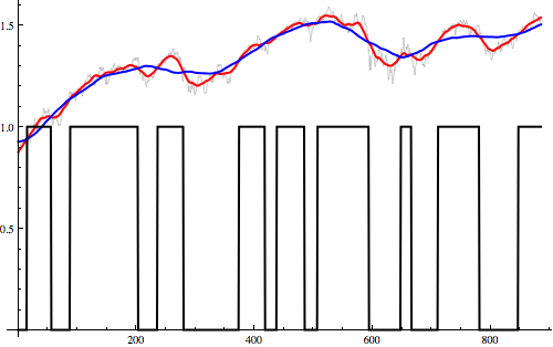
When the black line goes to 1 this signals that the short moving average has crossed over the long one meaning we should buy shares. When the black line drops to 0 this means we should sell. When do we know about this signal? The 120 day moving average needs data from +/- 60 trading days before and after the date you want to calculate the average for. This means you won’t know about a cross-over event until 60 days after the averages cross over. Shifting the signal gives the following:
signal = If[# >= 0, 1, 0] & /@ (ma30 - ma120);(*1 for hold,0 for sell*)
signal = Append[Drop[PadLeft[Drop[signal, -60], Length[ma120]], -1], 0];(*shift forward*)
graph = ListLinePlot[{((#/First[#]) &@ma1 - 1), signal},
  PlotStyle -> {{Black, Thin}, {Red, Thick}, {Blue, Thick}, {Black, Thick}}, ImageSize -> {500}]
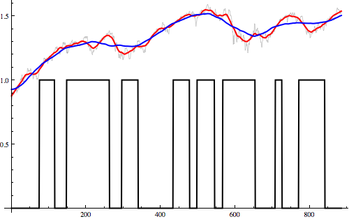
We can easily calculate the profit by calculating the difference of the signal with itself delayed one day. This produces a function that is 1 on buy days, -1 on sell days and 0 otherwise. Taking the product of this signal with the index price gives:
signal = If[# >= 0, 1, 0] & /@ (ma30 - ma120);(*1 for hold,0 for sell*)
signal = Append[Drop[PadLeft[Drop[signal, -60], Length[ma120]], -1], 0];(*shift forward*)
signal = MapThread[#2 - #1 &, {signal, Drop[Append[signal, 0], 1]}];(*turn into spikes 1 for buy,-1 for sell*)
profit = Accumulate[-signal*((#/First[#]) &@ma1)];(*calculate profit*)
graph = ListLinePlot[{((#/First[#]) &@ma1 - 1), profit},
  PlotStyle -> {{Black, Thick}, {Red, Thick}}, ImageSize -> {500}]
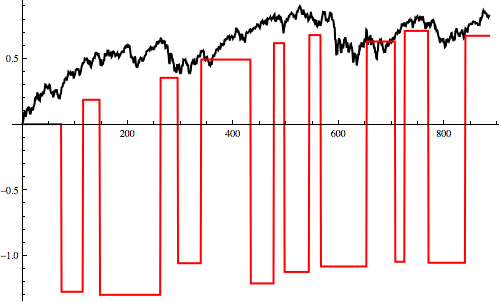
In the above chart, the red line shows how much cash we have and the black line shows the index for that period. We can see that although we make a 67% profit with our trading strategy, just investing in the index itself would have returned 83% – far better. Let’s see if we can improve that by adjusting the moving average sizes:
Instead of using an index this time, we’ll use individual stocks. We can define a function that takes two moving average sizes and returns the profit from using the moving average strategy as follows:
StrategyProfit[shortMA_, longMA_, clip_, series_] := Module[{
    x1 = Drop[(#/First[#]) &@ClippedMovingAverage[1, clip, series], 1],
    xshort = Drop[ClippedMovingAverage[shortMA, clip, series], -1],
    xlong = Drop[ClippedMovingAverage[longMA, clip, series], -1]},
  signal = If[# >= 0, 1, 0] & /@ (xshort - xlong);
  signal = Append[Drop[PadLeft[Drop[signal, -Floor[longMA/2]], Length[xlong]], -1], 0];
  signal = MapThread[#2 - #1 &, {signal, Drop[Append[signal, 0], 1]}];
  Return[Last[Accumulate[-signal*x1]]]]
Notice the argument “clip” - this corresponds to the longest moving average we’ll look at and helps avoid the problem that when we look at longer moving averages we have less data points to consider (because it takes a few points before the moving average can “start”). As an example with Microsoft using data from 2001-01-01 till now we get the following:
dateRange = {"2001-01-01", "2012-12-30"};
msft = Clean[FinancialData["MSFT", dateRange]];

StrategyProfit[30, 60, 60, msft]
> 0.251542
This tells us that using a 30-day/60-day moving average strategy would have given us a 25% RoI for the strategy compared to 39% for simply investing in MSFT directly – still not very good!
Edit: Jack pointed out in the comments that this actually returns -59% so it looks like I made a mistake with my date ranges here.. the 30/60 strategy is actually much much worse than I thought for the {“2001-01-01”, “2012-12-30”} date range.
Optimising the Strategy
Let’s exhaustively search the space of moving average sizes to see if we can do better:
FindBest[series_] := Module[
    {best = -1000, bestLong = 4, bestShort = 3},
    For[long = 10, long  best,
      best = profit; bestLong = long; bestShort = short;
      ]]
    ];
    Return[{bestShort, bestLong, best, InvestProfit[200, series]}]];
I’ve used exhaustive searching rather than Mathematica’s numerical optimisation functions like NMaximize here since it isn’t too costly to simply check all days and also the function is very jagged with many local maxima, making algorithmic search difficult (whether by simulated annealing, genetic algorithm or otherwise).
FindBest[msft]
> {8, 17, 1.08346, 0.0775735}
This tells us that using an 8/17 strategy, looking at the 8-day and 17-day moving averages, gave a return of 108% over the period compared to 8% for simply investing in MSFT directly. Lets look at some other stocks and see if we can find some strategies that consistently work. The Dow Jones Industrial Average currently has 23 stocks which have price information as far back as 2001:
symbols = StringSplit["MMM AA AXP T BA CAT KO DD XOM GE HPQ HD INTC IBM JNJ JPM MCD MRK MSFT PG UTX WMT DIS"];
dateRange = {"2001-01-01", "2012-12-30"};
prices = Clean[FinancialData[#, dateRange]] & /@ symbols;
We then write a quick script that will iterate through each stock and print the best strategy for each one. This takes some serious computation on my macbook, taking around half an hour to complete:
For[i = 1, i ", FindBest[prices[[i]]]]]
Once done we get the following results:
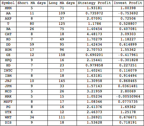
We can see that there is a huge variance in the best short and long moving average sizes to use. This is not good for our strategy. It suggests that our strategies are working more by luck than by any kind of intuitive understanding of the share price. This kind of makes sense because this kind of trading only depends on existing data - the price - we’re not actually adding anything new. The average short moving average length here is 16 days and the average long moving average length is 57 days. Lets see call this strategy 16/57 and see how it fairs if we use it in the 23 stocks chosen:
Mean[StrategyProfit[16, 57, 200, #] & /@ prices]
> 0.420134
Meaning that this strategy gives an average 42% return if we had used it for all 23 stocks from 2001 to now. And if we had instead just bought all those stocks?
Mean[InvestProfit[200, #] & /@ prices]
> 0.739597
…we would have made 74% profit! Not surprisingly, looking at moving average cross-overs fails to provide a winning strategy. It looks like I still have a long way to go before I can retire and let algorithms generate my income. Anyway, that’s all for this post. Cheers, Pete.